Indicators of Educational Development: Concept and Definition
Arun C. Mehta
- INTRODUCTION
- DIAGNOSIS OF THE EXISTING SITUATION
- THE PRESENT ARTICLE
- THE INDICATOR
- TYPES OF STATISTICS
- INDICATORS OF ACCESS (COVERAGE)
- ESTIMATES OF OVER‑AGE AND UNDER‑AGE CHILDREN
- OUT‑OF‑SCHOOL CHILDREN
- TRANSITION RATE
- INDICATORS OF EFFICIENCY
- INDICATORS OF FACILITIES
- CONCLUSIONS
- REFERENCES
INTRODUCTION
To achieve the goal of `Education for All’ envisaged in the National Policy on Education (1986) and its Revised Policy Formulations (1992), proper planning and effective implementation is required. Generally planning exercises are initiated at two levels, micro and macro levels of planning. In micro planning, plans are prepared at sub‑national level, such as, institution, village, block and district level, whereas macro plans are developed at the level which is just above the sub‑national level i.e. state and national level. At the district level, blocks, villages and educational institutions are units of micro planning but at the state level, district is an unit of micro planning. In India, barring a few states, educational planning is carried‑out at the state level, which do not ensure adequate participation of functionaries working at grassroots level. Of late, National Policy on Education (NPE, 1986 & 1992) and Eighth Plan envisaged disagregated target setting at least at the district level, which is also one of the major objectives of a number of projects and programmes currently under implementation in different parts of the country. Such programmes are IDA assisted District Primary Education Programme (DPEP), ODA assisted Andhra Pradesh Primary Education Project, UNICEF assisted Bihar Education Project (now under the ambit of DPEP), World Bank sponsored Basic Education Project in Uttar Pradesh (also under DPEP) and SIDA assisted Shiksha Karmi and Lok Jumbish projects in Rajasthan among of which the scope and coverage of DPEP is much more wider than other programmes of similar nature. The programme was first initiated in the year 1993 in 43 districts of seven states, namely, Assam, Haryana, Madhya Pradesh, Karnataka, Kerala, Tamil Nadu and Maharashtra. At present, the programme is under implementation in about 150 districts of fifteen states. Therefore, development of district plan at the district and lower levels with emphasis on participative planning is of recent origin.
DIAGNOSIS OF THE EXISTING SITUATION
There are different stages of planning but diagnosis of the educational development is one of the most important stages of planning. It is taking stock of the present situation with particular reference to different objectives and goal of `Education For All’ in general and `Universalisation of Elementary Education’ in particular. One of the other main objectives of the diagnosis is to understand district and its sub‑units with reference to educational development that has taken place in the recent past. Generally, cross‑sectional data for analysing existing situation and time‑series information for capturing trend is required, period of which depends upon the nature of a variable, which is to be extrapolated. The next important question is the level at which information need to be collected which depends upon the basic unit of planning.
Universal access to educational facilities is one of the important components of `Educational for All’; hence a variety of information relating to population of a village & habitation is required, so that school mapping exercises are undertaken. Exercises based on school mapping play an important role to decide location of a new school or whether an existing school is to be upgraded or closed down. Thus, number of villages distributed according to different population slabs is required so that opening of school in a habitation is linked to existing norms. In case of hilly and desert areas, the population norm of 300 is generally relaxed and lowered down. Habitations served by schooling facilities and whether they are available within habitation or a walking distance of one and three kilometers along with the total number of habitations in a district is also required, so as to assess the existing situation with reference to universal access. Similarly, percentage of rural population served by schooling facilities can also be used as an indicator of access, which should be linked to school mapping exercises. Similarly, information relating to adult learning and non‑formal education centers is required which should be analysed in relation to number of illiterates, out‑of‑school children and child workers.
Once the indicator of access is analysed, the next variable on which information is required is number of institutions. Within the institutions, the first important variable is availability of infrastructure in a school and its utilisation. Information relating to buildings, playgrounds and other ancillary facilities, such as, drinking water, electricity and toilets need to be collected and analysed. In other words, complete information relating to scheme of Operation Blackboard (MHRD, 1987) with reference to its implementation; adequacy, timely supply and utilisation need to be collected. Similarly, information relating to number of classrooms and their utilisation, class‑size, number of schools distributed according to class‑sizes and number of sections is also required which can be used in institutional planning related exercises.
Enrolment is the next important variable on which detailed information is required. Both aggregate and grade‑wise enrolment together with number of repeaters over a period of time needs to be collected separately for boys & girls, Scheduled Caste and Scheduled Tribe population, rural & urban areas and for all the blocks and villages of a district. The enrolment together with corresponding age‑specific population can be used to compute indicators of coverage, such as, Entry Rate, Net and Gross Enrolment Ratio, Age‑specific Enrolment Ratio and indicators of efficiency. Similarly, detailed information on number of teachers distributed according to age, qualifications, experience and subjects along with income and expenditure data is also required for critical analysis, so that optimum utilisation of the existing resources is ensured.
From the basic information, a variety of indicators can be generated which can be of immense help to understand a district and its sub‑units with particular reference to its demographic structure. It is not only the past and present information that is required but for proper and reliable educational planning, information on a few variables is also required in future. If the emphasis of planning exercises is on disaggregated target setting, then the entire set of statistics would have to be collected both at micro and macro levels of planning. The POA (1992) identified poor urban slum communities, family labour, working children, seasonal labour, construction workers, land‑less agricultural labour, forest dwellers, resident of remote and isolated hamlets as some of the target groups. Thus, information on these groups also need to be collected, if considerable size of a group(s) is concentrated in a district or its sub‑units.
It is not that all the data required for planning is available but information on a good number of variables may not be available. Generally, secondary sources are explored for diagnosis of the existing situation but for the variables, which are not available, primary data need to be collected. For example, age‑grade matrix is one such variable that is not readily available at the micro level but plays an important role in setting‑out-disaggregated targets. Hence, age‑grade matrix and other variables of similar nature is required for which sample surveys at the local level needs to be conducted and data generated. So far as the sources of data are concerned, Census publications for demographic and publications of State Education Department may be explored for educational data but the same may or may not be available in detail as required in the planning exercises. However, state‑wise information is available on most of the variables from the publications of the Department of Education, Ministry of Human Resource Development (MHRD) but latest publications are not available. For information relating to infrastructure, access, ancillary facilities and age‑grade matrix, NCERT publications may be explored but that is available only at a few points of time.
A variety of information relating to both general and educational scenario need to be collected. Information, such as on, geography, irrigation, transportation, industry and administrative structure is required, so as to prepare a general scenario of the existing infrastructure available in a district and its sub‑units. So far as the educational variables are concerned, required information can be grouped under information relating to demography, literacy and education sectors. Under the demographic variables, total population and its age and sex distribution separately in rural and urban areas need to be first collected. Apart from the total population, age‑specific population in different age groups is also required. For programmes relating to primary and elementary education, population of age‑groups 6‑10, 11‑13 and 6‑13 years and for adult literacy and continuing education programmes, population of age‑group 15‑35 years is required. Similarly, single‑age population (age `6′) is an another important variable on which information needs to be collected. In addition, information on a few vital indicators, such as, expectation of life at birth, mortality (death) rates in different age‑groups, fertility (birth) rate and sex ratio at birth is required so that the same can be used to project future population. For adult literacy and continuing education programmes, number of literate and illiterates in different age groups is required which should be linked to population in different age groups.
As soon as the diagnosis exercise is over, the next stage of planning needs review of past plans, policies and programmes implemented in the district with respect to its objectives, strategies and major achievements. It would be useful, if similar programmes are undertaken in future. (Mehta, 1997a). Generally, these programmes are related to promotion of education of Scheduled Caste and Scheduled Tribe, Girls and Total Literacy Campaigns. Reasons of failures and success of a particular programme need to be thoroughly analysed. If need be, the existing programme with or without modifications can be continued which should be followed by setting up of the targets on different indicators.
THE PRESENT ARTICLE
The variables identified for both general and educational scenarios cannot be used in its original form to draw inferences. Therefore, once the basic set of information is collected and complied, the next important step is to analyse data so as to derive meaningful indicators. The derived indicators are used to analyse different aspects of educational planning with particular reference to goal of ‘Education for All’ and can also serve as a decision support tool. Therefore, in the present article, the concept of an indicator and the methodology on which it is constructed is demonstrated by taking actual data at the all‑India level. If information on a particular variable is not available from the official sources, other agencies, like NCERT are explored and indicators computed. The indicators obtained are interpreted and its implications on the goal of ‘Education For All’ are also examined. In addition, the concept of an indicator and different types of statistics, such as, primary and secondary data, cross‑section and time‑series data and institution and stage‑wise data has also been discussed in length. More specifically, indicators on the following aspects of planning is constructed, developed and analysed :
(a) Coverage of Educational System
(b) Internal Efficiency of Education System and
(c) Quality of Services and its Utilisation.
Indicators on the above aspects can answer a variety of questions. System’s level of development, accessibility and children taking advantage of educational facilities are some of the questions, which relate to coverage of an education system. Thus, simple indicators like, enrolment ratio, entry rate, out‑of‑school and additional children need to enrol have been discussed. The next set of questions relates to internal efficiency of education system. Information on number of children who enter into the system and complete an education cycle, those who dropout from the system in between and number of children who reach to the next higher level can be obtained, if indicators of efficiency are computed. For this purpose, methods like, Apparent Cohort Method, Reconstructed Cohort Method and True Cohort Method have been discussed and indicators computed at the state and all‑India level. Similarly inequalities in the system, if any, can be detected and disadvantage group(s) be identified with the help of indicators of efficiency. The last set of questions relates to resources provided to education and how they contribute to the quality of educational services and whether resources being used in the most effective way possible, all of which answered efficiently, if indicators for disaggregated target groups are available. Time Utilisation Rate, Space Utilisation Rate, indicator of average audience in a class etc. are discussed under the group of quality of educational services and utilisation indicators.
THE INDICATOR
To understand what an indicator is and other questions of similar nature, let us first define an indicator itself. An indicator is that which points out or directs attention to something (Oxford Dictionary). According to Jonstone (1981), indicator should be something giving a broad indication of the state of the situation being investigated. The most common use of indicators is to examine the relative state of development of different systems accomplished over a period of time in a specified field of human concern (Prakash, Mehta and Zaidi, 1995). For example, primary enrolment of two districts do not produce any information but the same, if linked to corresponding age‑specific population, can be used to compare the status of primary education. In our day‑to‑day life we also come across various indicators which can be classified into three broad categories, namely, input, process and output indicators. Various process control machines, such as, videocassette recorder, automatic milk booths and automatic weighing machines are some of the examples of these indicators. However, in the field of education, the classification of indicators under different categories is not an easy task. Generally, we view education as a system, which receives inputs in the form of new entrants, transforms these inputs through certain internal processes, and finally yields certain outputs in the form of graduates. The output from a given cycle of education is defined as those students who complete the cycle successfully and the input used up in the processes of education are measured in terms of student years. These indicators can further be classified into four categories, namely, indicators of Size or Quantity, Equity, Efficiency and Quality, some of which are presented in Box 1.
TYPES OF STATISTICS
Before the concept and definition of a variety of indicators is presented, first the basic terms like, primary and secondary data, stage and institution‑wise data and stock and flow statistics is differentiated.
(i) Primary and Secondary Data
When information is first time collected, it is termed as primary data otherwise it is known as secondary data. Primary data is generally scattered in files, registers and records so as to collect it either from the concerned institutions or even can be collected from
BOX 1
BOX 1 |
|||
Selected Indicators of Educational Development |
|||
I Size |
II Equity |
III Efficiency |
IV
Quality |
| Enrolment Ratio
– Over-all Enrolment Ratio – Gross Enrolment Ratio – Net Enrolment Ratio – Age-specific Enrolment Ratio -Teacher-pupil Ratio – Admission Rate – Institutional: Pupil Ratio – InstitutionTeacher Ratio – Population Sex Ratio |
Coefficient of Equality between– Scheduled Castes – Scheduled Tribes – Male/Female – Rural/Urban Population |
Flow Rates– Promotion Rate– Drop-out Rate – Repetition Rate Internal Efficiency – Wastage Ratio – Input/Output Ratio – Transition Rate |
– Examination Results
– Percentage of students selected for national talent Search examination – Percentage of students qualified for IAS & other examinations – Percentage of students selected for CSIR/UGC fellowships/national testing etc. |
the sampling unit, such as, a teacher, school and student. The primary data is generally termed as raw which has no use to planners and decision making authorities, as it do not serve as a tool of decision support system. The information thus collected is processed, analysed and tabulated with the help of statistical indicators, so that it becomes derived information. Simple statistics, such as, averages, index numbers and growth rates can be used to generate derived data. The derived information in the form of indicators can also be used to analyse present status of educational facilities and its utilisation. At the micro level, just before beginning of an academic session, village survey is conducted. Generally, primary information on number of children in a specific age group and those who are out‑of‑school is collected which is an example of primary data. On the other hand secondary data generally lie in publications, which is readily available for use. Literacy rates during 1901‑91 that can be obtained from the Census publications is an example of secondary data.
(ii) Cross-sectional and Time‑Series Data
Generally two types of statistics, namely cross‑section and time‑series information is available. If information is available at a single point of time, it is known as cross‑sectional data. For example, state‑wise literacy rates and its male and female distribution in 1991 is an example of cross‑sectional data. Cross‑sectional data is also known as stock statistics. Stock statistics do not have flow of information and whatever is available that restrict to only a single point of time. On the other hand, information available on more than two points of time is known as time‑series information, which is also known as flow statistics. In flow statistics, there is a flow of information from one time period to another time period. State‑wise number of teachers during 1984‑85 to 1994‑95 is an example of time‑series data. Similarly, grade‑wise enrolment in 1991 is an example of stock statistics but if the same is also available for 1992, it becomes flow statistics. While analysing educational development, both types of statistics is needed. For projecting enrolment, we need enrolment over a period of time whereas for analysing present status of educational development, cross‑sectional data is required.
(iii) Institution and Stage‑wise Data
The third type of statistics generally we deal with is institution‑wise and stage‑wise information both of which can be cross‑sectional and/or time‑series in nature. For example, stage‑wise enrolment at the primary level includes all children those who are currently in primary classes irrespective of schools. Thus, while collecting stage‑wise information, enrolment irrespective of schools is considered. This means that primary stage enrolment includes enrolment in primary, middle, high and secondary schools. Otherwise, if consider enrolment in a particular type of school, it is termed as institution‑wise enrolment. Thus, enrolment in primary classes in primary schools is an example of institution‑wise data. In fact, a large number of children are in primary classes who are otherwise not in primary schools but are in middle and other higher levels of school education. Box 2 presents educational pattern in different States & UTs, which reveals that two types of patterns are in existence. In some states, primary level consists of Grades I‑V but in other states, it is Grades I‑IV. Similar is the case with middle and secondary levels of education. However irrespective of state patterns, the data disseminated in case of most of the publications covered Grades I‑V at the primary and VI‑VIII at the middle level.
BOX 2
|
BOX 2 |
|||
|
Educational Pattern in States & UTs STAGE |
|||
|
STAGE |
|||
|
State/UT |
Primary | Middle |
Secondary |
|
Andhra Pradesh |
I‑V | VI‑VII | VIII‑X |
| Assam | I‑IV | V‑VII |
VIII‑X |
|
Gujarat |
I‑IV | V‑VII | VIII‑X |
| Goa | I‑IV | V‑VII |
VIII‑X |
|
Haryana |
I‑IV | V‑VII | VIII‑X |
| Karnataka | I‑IV | V‑VII |
VIII‑X |
|
Kerala |
I‑IV | V‑VII | VIII‑X |
| Maharashtra | I‑IV | V‑VII |
VIII‑X |
|
Meghalaya |
I‑IV | V‑VIII | IX‑X |
| Mizoram | I‑IV | V‑VII |
VIII‑X |
|
Nagaland |
I‑IV | V‑VIII | IX‑XII |
| D & N Haveli | I‑IV | V‑VII |
VIII‑X |
| Lakshadweep | I‑IV | V‑VII |
VIII‑X |
Note : All other States & UTs have Grades I‑V and VI‑VIII corresponding to Primary and Middle levels of education.
Source : Annual Report: 1994‑95, MHRD, New Delhi.
INDICATORS OF ACCESS (COVERAGE)
In order to know whether the existing schooling facilities are equally available to clientele population/area/region or not, indicators of access are used. These indicators are also used to know whether schooling facilities are adequately utilised or not, because availability of school within a habitation or a walking distance need not guarantee that the entire clientele is utilising the facilities. While analysing accessibility, a number of indicators, such as, distance from the house, mode of travel and time need to reach schools are generally been used. While analysing, distance to travel to reach school, norms prescribed in policy can always be used. Generally, a primary school is supposed to be available within one kilometer from the habitation and a middle school within three kilometers. In India, habitations are treated as lowest unit of planning where schooling facilities should be available. Habitations are also known as cluster, which are below village level consisting of about ten houses. Thus, number of habitations having primary schooling facilities within a habitation and/or a walking distance is considered as an indicator of access, which if links to rural population, may generate more meaningful information. Thus, the second indicator of access one should consider is percentage of rural population served by the schooling facilities. For example about 94 percent of the total habitations in the country had schooling facilities either within the habitation or a walking distance of one kilometer which means that only six percent habitations were out of reach of schooling facilities. Similarly, about 95 per cent of the total population is being served by the schooling facilities which means that only a small segment of population is not accessible to schooling facilities. While developing plans at the micro level, the two indicators presented above should be computed separately for all of its sub-units. The identification of a habitation where schooling facilities are yet to be provided should be based on school mapping exercises referred above.
MEASURING THE EDUCATIONAL ACCESS
By measuring educational access, we mean interaction between demand and supply. Demand and supply in education means children of a specific age group utilising the educational facilities, which is termed as supply. Broadly, indicators of measuring educational access are the indicators of coverage. The following indicators of access are discussed in the present article:
(i) Admission Rate
(ii) Enrolment Ratio and
(iii) Transition Rate.
(i) Admission Rate
The first important indicator of educational access is Admission Rate which is also known as Entry or Intake Rate. Admission rate plays an important role to know coverage of child population (age 6’) in an education system, which is important to both policy makers and planners. When enrolment is analysed, we notice two types of children in Grade I i.e. new entrants and repeaters. But while computing the admission rate, only present members of cohort (new entrants, in Grade I are considered and repeaters are ignored, as they are members of some previous cohort. A cohort is simply a group element (children) moving together from one grade to another and from one time period to another. In some cases we may also have new entrants in other grades too, in situation like this we assume that their number is negligible. The admission rate plays an important role to know status of a district with respect to other districts of the state and can also be computed separately for boys & girls, rural and urban areas and Scheduled Castes & Scheduled Tribes population. The admission rate can be used to identify educationally backward blocks & districts, so that specific strategies are formed. As mentioned, admission rate also plays a significant role in enrolment projections and forms the basis of future enrolment in Grade II to VIII in subsequent years.
The computation procedure of Admission Rate is presented below:
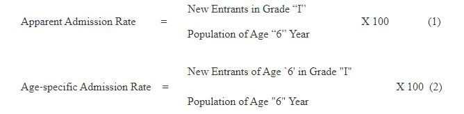
The admission rate presented above indicate that Apparent Admission Rate consider new entrants in Grade I irrespective of ages which means children above and below age `6′ are included in enrolment which may in some cases resulted into rate more than hundred. That is why the rate is known as Gross Admission Rate which is considered a crude indicator of access and may not present the true picture of the coverage. If considered total enrolment (Grade I) instead of new entrants, the corresponding rate is known is Gross Admission Rate which again is a crude indicator. Therefore, Age‑specific Admission Rate is computed which is considered better than the gross entry rate. Age‑specific admission rate cannot cross hundred because of its consideration of new entrants of age `6′ in Grade I which means children of below and above age `6′ are excluded from Grade I enrolment. This rate has serious policy implications and unless brought to hundred, the goal of UPE cannot be realised. Apart from the admission rate presented above, Cohort Admission Rate is last in the series which watch movement of a particular members of a cohort over several consecutive years and account for the member of cohort who successfully sooner or later enter school (Kapoor, n.d.) but due to limited data which is available on Grade I enrolment, the same cannot be computed at any level.
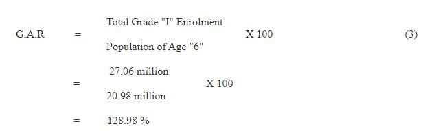
In 1990‑91, total enrolment in Grade I was reported 27.06 million including those of 1.23 million repeaters of previous cohort. The population of age `6’ officially entitled to get admission in Grade I was 20.98 million. Let us first compute Gross Admission Rate by using the following formula:
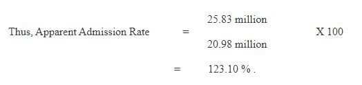
The computation of Apparent Admission Rate needs new entrants in Grade I which can be obtained by subtracting repeaters from the enrolment i.e. 27.06 ‑ 1.23 = 25.83 million.
The next rate, we compute below is Age‑specific Admission Rate which requires new entrants of age `6′ in Grade I which is readily not available from any of the regular sources. If we assume, 19.23 million children in Grade I of age `6′, then the Age‑specific Admission Rate is computed as follows:
which indicates that about 92 per cent population of age‑6 were admitted in schools or a little more than 8 per cent were otherwise out‑of‑school in the year 1990‑91. For some of the other cohorts, admission rate at the all‑India level is computed which is presented in Table 1 (Mehta 1993a & 1995a). The table reveals that a large number of children enter education system every year but it remains to see how many of them retain in the system. Further, it has been noticed that a large number of over‑age and under‑age children are also included in Grade I enrolment which makes the statistic more than hundred. Due to limitations in data, the net admission rate presented above couldn’t be computed.
Enrolment Ratio is the next indicator of coverage that is presented below.
Table 1
Apparent Admission Rate: All India
(1984‑85 to 1990‑91)
(Figures in Percentage)
|
Year |
Apparent | Admission | Rate | Gross Admission |
| Boys | Girls | Total |
Rate (Total) |
|
|
1984‑85 |
145.75 | 106.88 | 126.77 | 132.35 |
|
1985‑86 |
154.19 | 113.00 | 134.10 | 140.58 |
| 1986‑87 | 132.34 | 102.91 | 118.00 |
123.45 |
| 1987‑88 | 133.82 | 104.10 | 119.35 |
124.89 |
|
1988‑89 |
140.80 | 106.10 | 123.90 | 133.73 |
| 1989‑90 | 123.70 | 96.60 | 110.50 |
112.65 |
|
1990‑91 |
137.00 | 108.20 | 123.10 |
128.98 |
Note : Due to over‑age and under‑age children, the rate comes out more than 100 per cent.
Source : Mehta, Arun C. (1995a).
(ii) Enrolment Ratio: Concept, Definitions and Limitations
Enrolment Ratio is simply division of enrolment by population, which gives extent to which the education system is meeting the needs of child population. Two questions may crop‑up, first enrolment of which level and second, population of what age group. Before we present definition of enrolment ratio, let us first examine the position of different States & UTs with reference to enrolment ratio at primary and middle levels of education. It has been observed that in many of our states, the enrolment ratio at the primary level is more than 100 per cent (currently 105 per cent at the national level, Table 2) and on the other hand in some states like Bihar (76%), Rajasthan (91%) and Uttar Pradesh (89%); the enrolment ratio is less than hundred. Further, it has been observed that at the middle level, except for Himachal Pradesh, Kerala, Mizoram, Lakshadweep, Pondicherry and Tamil Nadu, none of the states have enrolment ratio more than hundred per cent which shows the quantum of drop‑outs from one stage to another and incidence of over‑age and under‑age children. It has also been noticed that in some of the smaller States & UTs, such as, Goa, Dadar and Nagar Haveli, Manipur, Mizoram, Sikkim, Lakshadweep and Pondicherry where the base population (age‑specific) is small, only slight over‑reporting of enrolment and over‑age and under‑age children dramatically change the enrolment ratio (Table 3). In order to understand statistics on enrolment, the following enrolment ratios are discussed in detail in the present article.
(A) Over‑All Enrolment Ratio
(B) Age‑Specific Enrolment Ratio and
(C) Level Enrolment Ratio.
The concept of different ratio is demonstrated by computing it at the primary and middle levels of education. The merits and limitations of a particular ratio is also discussed which may lead us to identify the best indicator of coverage. The indicator identified may thus help us to know the present position on different aspects of Education for All.
(A) Over‑All Enrolment Ratio
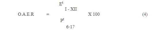
The first indicator of coverage we discuss below is Over‑All Enrolment Ratio (OAER) which presents an overall picture or a birds eye‑view of the education system under study. For a school system consisting of Grades I‑XII, the OAER is simply division of total enrolment in Grades I‑XII to population in the respective age‑group i.e. 6‑17 years (equation 4). It may be observed that in the numerator, total enrolment in Grades I‑XII is considered irrespective of ages, but in the denominator corresponding school‑age population i.e. 6‑17 years is considered which may sometimes lead to serious problems. In some cases, quantity in numerator may be higher than the quantity in the denominator, which gives enrolment ratio often more than 100 per cent. Technically, if the enrolment ratio for a particular stage in a block/district/state/country is 100 percent, it means that the goal of universal enrolment has been achieved but in reality the case is not so. When enrolment ratio is found to be more than 100 per cent, it may be due to over‑age and under‑age children which are included in enrolment of Grades I‑XII. Other possible reason of this may be due to large scale over‑reporting, may be intentional and/or unintentional, to show the fulfillment of targets which can be checked only, if average daily attendance is available. Thus, OAER is not considered an ideal indicator of enrolment and planning exercises based on it may lead to misleading picture. Hence, it is termed a crude indicator of coverage. The second important limitation of this ratio is that level and stage‑wise enrolment ratio cannot be obtained. The ratio is recommended to use only when quick estimates are required and detailed information on enrolment is not available.
Table 2
Gross Enrolment Ratio at Primary Level in Selected
States of India
1993‑94
(Figures in Percentage)
States |
Gross Enrolment Ratio |
||
| Boys | Girls | Total | |
| Andhra Pradesh | 116 | 100 | 108 |
| Arunachal Pradesh | 133 | 99 | 116 |
| Assam | 134 | 125 | 130 |
| Bihar | 96 | 54 | 76 |
| Gujarat | 131 | 126 | 119 |
| Himachal Pradesh | 127 | 112 | 119 |
| J and K | 104 | 73 | 89 |
| Karnataka | 124 | 115 | 120 |
| Kerala | 104 | 101 | 102 |
| Madhya Pradesh | 117 | 91 | 105 |
| Maharashtra | 124 | 115 | 119 |
| Manipur | 100 | 96 | 98 |
| Mizoram | 139 | 132 | 136 |
| Rajasthan | 120 | 61 | 91 |
| Sikkim | 124 | 111 | 118 |
| Tamil Nadu | 149 | 141 | 145 |
| Tripura | 141 | 119 | 130 |
| Uttar Pradesh | 104 | 73 | 89 |
| West Bengal | 125 | 123 | 124 |
| All India | 115 | 93 | 105 |
Source : Selected Educational Statistics: 1993‑94, Department of Education , MHRD, Government of India, New Delhi, 1994.
The total enrolment in Grades I‑XII and the corresponding population in the age‑group 6‑17 years in 1986‑87 was 128.22 million and 170.55 million (estimated) respectively (Table 5), thus giving an enrolment ratio of
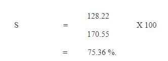
Enrolment ratio of 75.36 per cent means that more than seventy five per cent of the total 175.55 million children of the age‑group 6‑17 years including over‑age and under‑age children were enrolled in 1986‑87.
Table 3
Enrolment (Grades I‑V) and School‑Age Population (6‑11 Years)
in Smaller States/UTs: 1993‑94
(Figures in Hundred)
| States | Population | Enrolment | ||
| (6‑11 years) | (I‑V Classes) | |||
| Girls | Total | Girls | Total | |
| Dadar and Nagar Havelli | 89 | 170 | 75 | 187 |
| Goa* | 676 | 1350 | 634 | 1324 |
| Lakshadweep | 31 | 62 | 40 | 88 |
| Manipur | 1185 | 2458 | 1138 | 2245 |
| Mizoram | 414 | 853 | 548 | 1157 |
| Pondicherry | 374 | 754 | 500 | 1056 |
| Sikkim | 316 | 639 | 351 | 752 |
* ‑ Includes Daman and Diu
Source : Same as Table 2.
(B) Age‑Specific Enrolment Ratio
The second ratio we discuss below is Age‑Specific Enrolment Ratio (ASER). It gives enrolment ratio for a particular age or age group. It is simply division of enrolment in year `t’ in age‑group `a’ in all the levels of education in any grade by a population of a particular age `a’ in that year `t’. The limitation of the ASER is that it consider total enrolment irrespective of its ages, hence enrolment in numerator is not free from error, as it consists of enrolment in different grades. Still, ASER may be useful to planners and policy makers when information on coverage and children not enrolled in a particular age group is required.
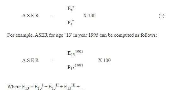
Similarly, Age‑specific enrolment ratio can be obtained for any other single age or age‑group. For example, in 1986‑87 total enrolment of age‑group 6‑10 and 11‑13 years was 71.11 and 29.11 million respectively (Table 5) which if divided by the corresponding age‑specific population i.e. 93.70 and 56.88 million, gives
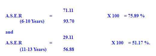
Thus, of the hundred children of age‑group 6‑10 and 11‑13 years, about 75.89 and 51.17 per cent were in the system but the enrolment data shows that a good number of children belong to grades other than I‑V and VI‑VIII. In fact, children of age‑group 6‑10 years are expected to be in Grades I‑V, if school entrance age is strictly restricted to age `6′ but the situation in reality is not so. Similar is the case with children of age‑group 11‑13 years in Grades VI‑VIII.
The next ratio we present below is Level Enrolment Ratio.
(C) Level Enrolment Ratio
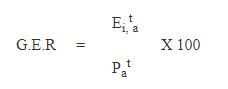
The Level Enrolment Ratio is an improved version of OAER, which gives enrolment ratio level‑wise. Two types of ratios, namely, `Gross and Net’ enrolment ratios are available. The Gross Enrolment Ratio (GER) is a division of enrolment at school level `i’ in year `t’ by a population in that age group `a’ which officially correspond to that level `i’.
On the basis of above formula, GER for primary and middle levels of education in any given year, say 1987 can be computed as follows:
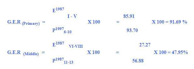
Again, it has been observed that GER includes over‑age and under‑age children in enrolment which often resulted into enrolment ratio more than hundred and the same should not be used in planning exercise unless the net amount of children in the respective age‑group is considered. Net Enrolment Ratio (NER) is an improved version of the GER. The difference between GER and NER is in its consideration of enrolment (equation 7). In NER, over‑age and under‑age children are excluded from enrolment and then ratios to the respective age‑specific population are obtained. One of the limitations of the NER is that it excludes over‑age and under‑age children from the enrolment though they are very much in the system. Despite these limitations, the ratio seems to be more logical than the other ratio presented above.
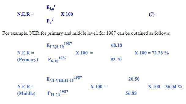
The GER and NER computed above at the primary level comes out to be 91.69 and 72.76 per cent respectively which indicate that about 18.93 per cent children were from out‑side the prescribed age‑group i.e. 6‑10 years. Compared to primary level, the percentages of over-age and under-age children at the middle level were low at 11.91 per cent. But, computation of NER requires data on age‑grade matrix, which, as mentioned, is not -available. Thus, GER is the only indicator of enrolment which is available annually apart the age‑specific ratio from the Census sources. However, few estimates of over‑age and under‑age children at the school level are available which are briefly presented below.
ESTIMATES OF OVER‑AGE AND UNDER‑AGE CHILDREN
The estimates of over‑age and under‑age children at the primary and middle levels of education are available most of which are computed at the all‑India level, only few are available at the state level. In order to compute number of children outside the prescribed age‑group, information on under‑age and over‑age children is required but the available estimates cannot be used directly at the block, district and state level because of the methodology used in generating estimate vary from source to source. At the elementary level, the most authentic source of grossness is the Ministry of Education (MOE) estimate which is based on the actual age‑grade matrix but the same is available only up to the year 1970‑71, after that the series was discontinued. Using the MOE age‑grade data during the period 1950 to 1970 and by employing Method of Least Squares, Kurrien (1983) estimated 22 per cent as an amount of grossness at the primary level and 39.2 per cent at the middle level.The next source of grossness that is also based
Table 4
Estimate of Over‑age and Under‑age Children at Different Levels of
Education : NSS0 42nd Round (July 1986 ‑ June 1987)
(Figures in Percentage)
|
Educational Level |
Rural | Urban | Total | ||||||
|
|
Boys | Girls | Total | Boys | Girls | Total | Boys | Girls | Total |
|
Primary |
23.87 | 22.71 | 23.43 | 24.74 | 24.21 | 24.50 | 24.08 | 23.15 |
23.71 |
| Middle | 18.15 | 13.77 | 16.84 | 14.14 | 12.66 | 13.48 | 17.08 | 13.32 |
15.78 |
| Elementary | 22.18 | 20.69 | 21.64 | 21.33 | 20.49 | 20.96 | 21.96 | 20..62 |
21.45 |
Source : Mehta, Arun C.(1993b).
on complete enumeration of educational institutions like the MOE estimate, is the NCERT estimate but that too is available occasionally, 1986‑87 being the latest one (recently, it is also made available for 1993-94). The estimate is based on survey data, which provides age-grade matrix only at the all-India level, and no information is available at the state level. Kurrien estimate of 22 per cent at primary level is amply supported by the MOE and NCERT estimates. A number of other estimates based on sample surveys are also available which is provided by NIEPA (1992 & 1993) and NSSO (1991). But, due to small size of sample, the estimate of grossness cannot be generalised at the all‑India and even at the state level. The estimates of over‑age and under‑age children are also referred and used in the Working Group on Early Childhood and Elementary Education (1989), Eighth Five Year Plan document (1992) and EFA document of MHRD (1993a) but are available only at the all‑India level. While, the working group used 22 per cent as an estimate of total grossness at all levels of education, the Eighth Plan used only 15 per cent compared to 25 per cent referred in EFA document. Also, reference has been not been given on the basis of which the estimates are computed. Hence, the estimates can be best used at the all‑India level only.
The next estimate, which is available separately for rural and urban areas, is the NSSO estimate based on the household survey conducted during 1986‑87. Like NCERT estimate, it is also available at a single point of time and that too at the all‑India level only, hence no time‑series can be built‑up. The NSSO estimate compares well with the MOE and NCERT estimates especially at the primary level, however, a significant difference has been noticed at the middle level. Thus, MOE estimate at the state level and NCERT and NSSO estimates are left for use at the all‑India level. However, these estimates are too outdated to use but in the absence of the latest data, there is no option but to use the available estimates in whatsoever form they are available. In addition, the estimate of grossness can also be derived from the states where enrolment ratio (gross) at present is more than hundred per cent. A perusal of 1993‑94 enrolment ratio reveals that in a number of States & UTs it is very high. For instance Tamil Nadu (145.00%), West Bengal (123.90%), Maharashtra (119.40%), Karnataka (119.90%), etc. had very high enrolment ratios, which means at least 45.00, 23.90, 19.40 and 19.90 per cent grossness at the primary level. Further, it has also been noticed that enrolment targets at the state level provided in the Eighth Plan document when added together do not matches well with the targets fixed at the all‑India level and the deviation is significant, hence pro‑rata adjustment is required which means the estimate of grossness at the all‑India level may not be applicable at the state level. At the micro‑level, especially at the block and district level, where setting‑up of targets is an important task, needs estimates of over‑age and under‑age children. The available estimates of all‑India level cannot be used at the micro‑level, for that purpose, a survey at the local level would be most appropriate to conduct. However, out‑of‑school children in the present article is computed on the basis of NSSO estimates (Table 4) i.e. 24.1, 17.1 and 21.9 per cent for boys and 23.2, 13.3 and 20.6 per cent for girls are considered estimates of over‑age and under‑age children respectively at the primary, middle and elementary levels of education.
Table 5
Age and Grade Distribution of Enrolment and Population
NCERT Fifth Survey: 1986‑87
| AGE‑GROUP | ||||
| Grade | 4 to Below 6 Years | 6 to Below 11 Years | 11 to Below 14 Years | Total |
| (1) | (2) | (3) | (4) | (5) |
| I | 10309502 | 14439597 | 134028 | 24890467 |
| II | 738263 | 17122286 | 381266 | 18254892 |
| III | 16486 | 15685139 | 652049 | 16385969 |
| IV | 1830 | 12716348 | 1289112 | 14085382 |
| V | ‑ | 8221306 | 3897978 | 12296768 |
| I to V | 110066081 | 68184676 | 6354433 | 85913478 |
| VI | ‑ | 2493112 | 7519761 | 10501690 |
| VII | ‑ | 354253 | 7580324 | 8918548 |
| VIII | ‑ | 75931 | 5403436 | 7852098 |
| VI‑VIII | ‑ | 2923296 | 20503521 | 27272136 |
| IX | ‑ | ‑ | 1880968 | 6408929 |
| X | ‑ | ‑ | 367193 | 5111057 |
| XI | ‑ | ‑ | ‑ | 2106586 |
| XII | ‑ | ‑ | ‑ | 1402985 |
| I to XII | 110066081 | 71107971 | 29106414 | 128215381 |
| Population | ‑ | 93697824 | 56881290 | ‑ |
Source: Fifth All India Educational Survey, NCERT, New Delhi, 1993.
OUT‑OF‑SCHOOL CHILDREN
The estimate of over‑age and under‑age children also plays an important role to work‑out out‑of‑school children which is an important component of planning exercise It has been noticed that in most of our planning exercises, out‑of‑school children are conspicuous by their absence and additional children need to enroll is only computed which is also not free from limitations. The detailed procedure of computing out‑of‑school children is presented in Box 3 which is based on the data of Sixth All India Educational Survey for year 1993‑94. For obtaining out‑of‑school children, first enrolment is refined with particular reference to estimate of over‑age and under‑age children. Thus, the corresponding percentage of over-age and under-age children have been taken‑out from enrolment and the refined enrolment is obtained. The balance of age‑specific population and refined enrolment is termed as out‑of‑school children. For demonstration purposes, out‑of‑school children is computed only for Primary Level/Age‑group 6‑10 years,
Box 3
Computation of Out‑of‑School and Additional
Children Need to Enroll
(Based on NCERT Data)
(In Million)
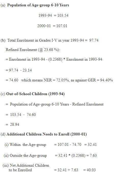
otherwise the same needs to be computed separately for boys and girls, Scheduled Caste & Scheduled Tribe children and rural & urban areas. If computed at the disaggregated levels, the same will help to identify educationally backward areas where out‑of‑school children concentrate, so as to adopt appropriate strategies to bring them under the umbrella of education.
The out‑of‑school children computed indicate a net enrolment ratio of 72.05 per cent as against 94.40 per cent gross enrolment ratio which means that only 72 per cent of the total 103.54 million children of the age‑group 6‑10 years were enrolled in 1993-94. The existing data do not allow us to know how many of them were actually attending schools regularly which can be known only, if average daily attendance is available. The out‑of‑school children is also used to project additional number of children need to enroll over a period of time, if goal of universal enrolment is to be realised. For projecting additional children, projected population of the respective age‑group in the target year i.e. 2001 is required. The results (Box 3) indicate that for achieving goal of universal enrolment about 40 million additional children in the age group 6‑10 will have to be enrolled by the year 2001.
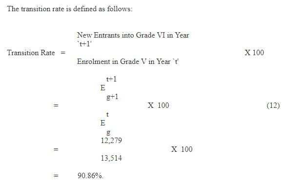
TRANSITION RATE
The next indicator of coverage is Transition Rate, which is based on `Student Flow Analysis’. Before we present the concept of transition rate and its computation procedure, it is better first to discuss student flow analysis and different flow rates, which are presented below.
(A) Student Flow Analysis
Student Flow Analysis starts at the point where students enter into an education cycle. The flow of student into, through and between an educational cycle is determined by the following factors (UNESCO, 1982):
I : Population of Admission Rate (`6′ Year)
II : Student Flow into the System : The Admission Rate
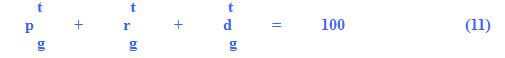
III : Student Flow through the System : Promotion, Repetition and Drop‑out Rates and
IV : Student Flow between Systems : The Transition Rate.
The rates mentioned above are important to understand the education system which can also answer a variety of typical questions, such as, at which grade in the cycle is the repetition or drop‑out rate highest?, who tends to drop‑out and repeat more frequently boys or girls? and what is the total, accumulated loss of students through drop‑out?. The answer of these questions can be obtained, if flow rates for different target groups and for each grade are computed. The transition of students between cycles has, of course, a great significance of its‑own. It is not in planners hand that he/she will control different flow rates but through policy interventions they can be altered over a period of time.
Since, the concept and definition of Admission Rate is already presented in the last section, we start student flow analysis by assuming that a student has already entered into the system and there are now only following three possibilities in which he/she will move:
- Students have been promoted to the next higher grade
- Students have to repeat there grades and
- Students have dropped‑out from the system.
In the educational statistics, it is convention that enrolment is presented in a rectangle box, which has three directions each of which indicate flow of students. The diagonal indicate flow of students who successfully complete a grade and are now promoted to next higher grade. While down below direction represents number of children who repeat a particular grade but only in the next year. The last direction indicates the balance of those who are neither promoted nor repeated and are termed as dropouts from the system without even completing a particular grade (Figure 1).
For convenience point of view, total enrolment in Grade I is considered 1,000. It may be noted that total of promotees, repeaters and dropouts are equivalent to enrolment in a particular grade. In order to workout flow rates, grade‑wise enrolment for at least two consecutive years along with number of repeaters is required. If information on number of repeaters is not available, the flow analysis is based on Grade Ratios, which is also known as pass percentage. Grade Ratio is simply division of enrolment in the next grade (say Grade II) to enrolment in the previous grade (say Grade I) in the previous year. Since, enrolment is not free from limitations because of the repeaters, the method may not present the true picture of the existing situation. Hence, Grade
Flow Diagram (I)
Figure 1
Ratio is termed a crude indicator of promotion rate. If number of repeaters is available, the analysis is based on promotion rate which is bound to be more reliable than based on the Grade Ratio. The method also assumes that transfer from a school to another school within or outside a block/district is negligible. In case, if their number is significant, they should be considered in calculation, otherwise the same can produce unrealistic rates. Below the detailed procedure of calculation of flow rates is demonstrated by considering actual set of data presented in Box 4. Grade‑wise enrolment along with number of repeaters at the all‑India level is used for years 1989‑90 and 1990‑91.
(a) Promotion Rate
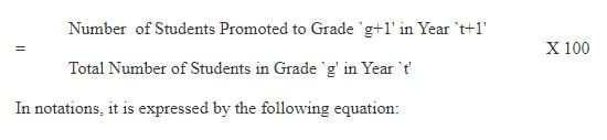
The first rate we discuss below is promotion rate, which needs to be computed separately for all the grades. The main task is to obtain number of promotees who are promoted to next grade. Of the total 23,592 thousand children in Grade I in 1989‑90, it look like that about 20,999 thousand children were promoted to the next higher grade i.e. Grade II in 1990‑91. But in reality, the number of promotees was 20,401 and not 20,999 thousand because of 598 thousand repeaters who were also included in Grade II enrolment, which needs to be taken out from enrolment. Thus, the actual number who were promoted to Grade II in 1990‑91 was 20,999 ‑ 598 = 20,401 thousand. In the similar fashion, promotees in the remaining grades are to be worked out. Once the number of promotees is worked out, the next step is computation of promotion rate in different grades. Thus, promotion rate in a particular grade can be computed as follows:
BOX 4
Enrolment and Repeaters at the All India Level
1989‑90 & 1990‑91
(In Thousand)
| Year | GRADES | Total | |||||||||
| I | II | III | IV | V | I‑V | VI | |||||
| Enrolment | |||||||||||
| 1989‑90 | 23,592 | 22,019 | 17,832 | 15,394 | 13,514 | 92,351 | 11,862 | ||||
| 1990‑91 | 27,062 | 20,999 | 18,866 | 16,152 | 14,296 | 97,375 | 12,913 | ||||
| Repeaters | |||||||||||
| 1989‑90 | 1,005 | 606 | 719 | 688 | 668 | 3,686 | 1,109 | ||||
| 1990‑91 | 1,230 | 598 | 576 | 628 | 571 | 3,603 | 634 | ||||
| Flow Diagram | |||||||||||
| Year | I | II | III | IV | V | VI | |||||
| 1005 | 606 | 719 | 688 | 668 | |||||||
| 1961 | 3131 | 1732 | 1041 | 664 | |||||||
| 1989‑90 | 23592 | 22019 | 17832 | 15394 | 13514 | 11862 | |||||
| 1230 | 598 | 576 | 628 | 571 | 634 | ||||||
| 20401 | 18290 | 15524 | 13725 | 12279 | |||||||
| 1990‑91 | 27062 | 20999 | 18866 | 16152 | 14296 | 12913 | |||||
| Flow Rates (%) | |||||||||||
| I to II | II to III | III to IV | IV to V | V to VI | |||||||
| Promotion | 86.47 | 83.06 | 87.06 | 89.16 | 90.86 | ||||||
| Repetition | 5.21 | 2.72 | 3.23 | 4.08 | 4.23 | ||||||
| Drop‑out | 8.31 | 14.22 | 9.71 | 6.76 | 4.91 | ||||||
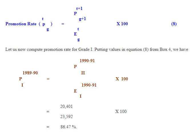
Thus, 86.47 per cent promotion rate in Grade I indicates that the remaining 13.53 per cent children were either dropped‑out from the system and/or repeated Grade I next year. By adopting the same procedure, promotion rate in remaining grades can also be computed (Box 4).
(b) Repetition Rate
Once the promotion rate is computed, the next indicator that is required to compute is grade‑to‑grade repetition rate. Since the number of repeaters is already given, the computation of repetition rate is as simple as division of number of repeaters in a grade to enrolment in the previous year in the same grade. The Box 4 presents complete analysis of student flow which has repeaters for two consecutive years, namely 1989‑90 and 1990‑91. Care should be taken to select one out of them. For computing repetition rate in a grade, say Grade I in 1989‑90, repeaters of 1990‑91 is considered because a repeater can repeat a particular grade only in the next year. In notations, it is presented as follows:
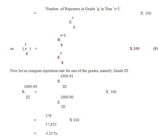
Thus, the repetition rate in Grade III indicates that of the 17,832 thousand children in 1989‑90, only 3 per cent repeated next year. The remaining children may be either promoted to Grade IV or they were dropped‑out from the system before completion of Grade III.
Similarly repetition rate in any other grade can also be worked‑out.
(c) Drop‑out Rate
One of the important indicators of educational development is dropout rate which like other rates should be computed grade‑wise. Before the dropout rate is computed, the first requirement is to obtain number of dropouts between the grades. In the last two steps, we have calculated number of promotees and repeaters in different grades. In fact, the balance of enrolment in a particular grade is termed as drop‑outs. Or in other words, of those who are not promoted and/or repeated is known as drop‑outs. For example, Grade I enrolment in 1989‑90 was 23,592 thousand of which 20,401 children were promoted to next higher Grade II and 1,230 thousand children repeated Grade I which means, the resultant 23,592 ‑ 20,401 ‑ 1,230 = 1,961 is termed as dropouts of Grade I. The number of dropouts can now be easily linked to enrolment in a particular grade and dropout rate can be obtained. First the formula is presented:
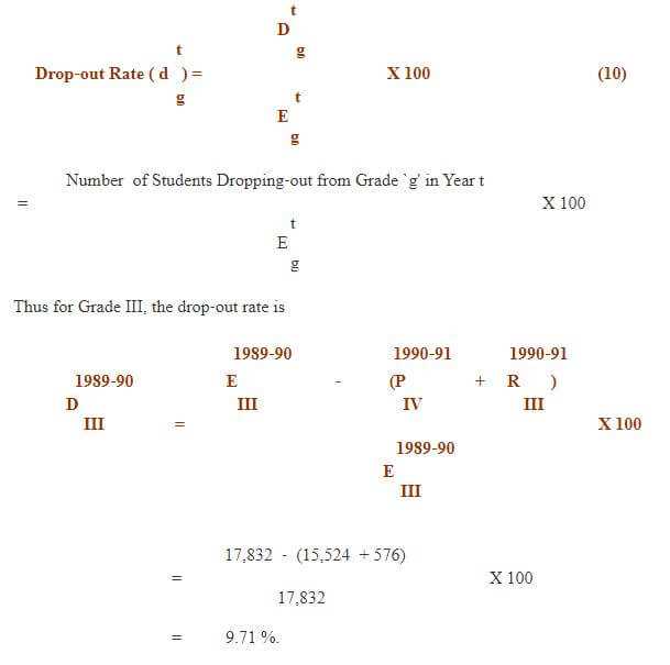
Drop‑out rate in Grade III indicate that about 9.71 per cent children of those who were in Grade III in 1989‑90 dropped‑out from the system without completing Grade III, thus contributing a lot to wastage of resources.
It should however be noted that addition of promotion, repetition and drop‑out rates in a particular grade is always 100 per cent. Knowing two of them means knowing the third one as well.
The different flow rates presented above also play an important role when exercise of internal efficiency of education system is undertaken which cannot be obtained unless, flow rates are available. However, educational planner and policy makers are particularly interested in those successful who proceed to the next higher cycle. In order to trace the flow of students from one cycle to other; Transition Rate is very useful. The transition of students between cycles has, of course, a great significance of its own. It can be manipulated for purposes of educational policy. After a student is reached at the final grade i.e. Grade V, or Grade IX or Grade XII, there are the following four possible ways in which they move (Figure 2):
(i) a student may repeat the grade
(ii) a student may drop‑out from the system
(iii) a student may complete the grade successfully and then leave the school system and
(iv) a student may complete the grade successfully and then enrol in the first grade of the next higher cycle.
Flow Diagram (II)
Text Box: Drop‑outs (50)
Text Box: Enrolment in Final Grade
of a Cycle
1000 Students
Text Box: Successful Completors Who Continue in Grade I of Next Higher Cycle (350)
Text Box: Successful Completors Who Have Left the System (500)
Text Box: (Repeaters) (100)
Figure 2
With the limited set of data, it is not possible to exactly know successful completors who continue in Grade I of next higher cycle. The transition rate, thus computed is nothing but the promotion rate between final grade of a cycle and first grade of next cycle. The number of drop‑outs so calculated consists of both who complete the cycle successfully but not taken admission in the next cycle and also who dropped‑out in between without completing the last grade of first cycle.
In the present article, for demonstration purposes transition rates have been calculated (1985‑86) for primary to middle and from middle to secondary levels of education. Table 6 reveal that at the all‑India level, out of hundred children in Grade V, only 83 could take admission in Grade VI as compared to 78 girls, which means in transition 17 per cent children dropped‑out from the system as compared to 22 per cent girls which also included fresh admissions to Grade VI. The state‑wise results reveal that from primary to middle level, the transition rates vary from 55.79 per cent in Nagaland to 92.48 per cent in Karnataka for total enrolment compared to 54.23 per cent in Nagaland to 91.38 per cent in Tripura for girls enrolment. Karnataka (92.48%) had the highest transition rate which is followed by Maharashtra (89.78%), Punjab (90.34%), Haryana (87.09%), Tripura (91.79%) and Uttar Pradesh (86.32%). The transition rates for Maharashtra and Tripura are included that of the repeaters, hence may not present the correct picture.
It has also been revealed that during transition, about 28.67 per cent (Sikkim), 18.3 per cent (Andhra Pradesh), 26.58 per cent (Orissa) and 27.59 per cent (Gujarat) children dropped‑out from the system. In Kerala too, about 16.20 per cent children dropped‑out during the transition compared to 13.46 per cent girl children. In Jammu & Kashmir, the rate so calculated is not reliable as it comes out to be 100.91 per cent, similar is the case with Meghalaya.
The transition rate from middle to secondary level calculated at the all‑India level shows that of 100 students in Grade VIII, only 77 could take admission in Grade IX which means more than 23 per cent students dropped‑out from the system during the transition as compared to 25 per cent girls. The state‑wise analysis also present grim situation where as many as 54.58 per cent (Himachal Pradesh), 47.95 per cent (Sikkim), 25.47 per cent (West Bengal), 19.30 per cent (Gujarat), 44.36 per cent (Madhya Pradesh) etc. children dropped‑out from the system in transition. But at the same time, Karnataka had only 3.47 per cent drop‑outs followed by Tripura (4.22%), Rajasthan (7.95%), Nagaland (8.23%) and Maharashtra (8.80%). On the other hand, Kerala one of the educationally advanced state had about 23 per cent children whom dropped‑out during the transition, as compared to 21 per cent girls.
Table 6
Transition Rates at Primary and Middle Level
of Education: 1985‑86
(In Percentage)
| States | Primary to Middle | Middle to Secondary | ||
| Stage | Stage | |||
| Total | Girls | Total | Girls | |
| Andhra Pradesh | 71.69 | 64.96 | 75.09 | 74. 79 |
| Assam | 78.33 | 76.33 | 78.18 | 81.49 |
| Bihar | 78.22 | 70.81 | 82.17 | 70.86 |
| Gujarat | 72.41 | 69.43 | 80.70 | 81.20 |
| Haryana | 87.09 | 80.04 | 58.56 | 58.09 |
| Himachal Pradesh | 84.26 | 79.93 | 45.42 | 42.42 |
| Jammu & Kashmir* | 100.91** | 98.37 | 97.97 | 101.75 |
| Karnataka | 92.48 | 88.24 | 96.53 | 96.29 |
| Kerala | 83.80 | 86.54 | 76.59 | 78.92 |
| Madhya Pradesh | 82.34 | 73.95 | 55.64 | 48.66 |
| Maharashtra* | 89.78 | 88.77 | 91.20 | 89.18 |
| Manipur | 75.19 | 77.91 | 79.59 | 79.28 |
| Meghalaya | 75.52 | 84.74 | 101.81** | 102.66** |
| Nagaland | 55.79 | 54.23 | 91.73 | 91.00 |
| Orissa | 73.42 | 65.96 | 81.60 | 74.69 |
| Punjab | 90.34 | 84.72 | 75.16 | 74.46 |
| Rajasthan | 98.85** | 85.16 | 92.05 | 84.45 |
| Sikkim | 71.33** | 70.76 | 52.05 | 51.21 |
| Tamil Nadu | 84.15 | 75.68 | 81.23 | 75.25 |
| Tripura* | 91.79 | 91.38 | 95.78 | 94.87 |
| Uttar Pradesh | 86.32 | 75.59 | 74.53 | 63.54 |
| West Bengal* | 75.85 | 75.59 | 74.53 | 63.54 |
| All India | 83.18 | 77.94 | 77.40 | 74.52 |
* Including repeaters
** Excluding Repeaters, but data not reliable
Source :Mehta, Arun C. (1995b).
INDICATORS OF EFFICIENCY
Despite spectacular quantitative expansion of educational facilities in the country, the desired level of achievement with respect to coverage, retention and attainment couldn’t be achieved mainly due to low level of efficiency upon which the system is currently based. Though, a number of common indicators of efficiency presented above are computed widely both at the state and all‑India level, still a number of other indicators considered to present more reliable picture of internal efficiency of education system are generally not computed largely due to their lengthy computation procedure. Therefore, an attempt has been made in the present article to demonstrate how different indicators of wastage and status of internal efficiency of education system are measured and computed. Broadly, the following methods are discussed in detail:
(a) Apparent Cohort Method
(b) Reconstructed Cohort Method and
(c) True Cohort Method.
(a) Apparent Cohort Method
The simple but crude method of measuring extent of educational wastage which require minimum amount of information is Apparent Cohort method. The method requires either cross‑sectional (year‑grade) or time‑series data on grade‑wise enrolment both of which is easily available on fairly a long period. If the cross‑sectional grade data is considered, the percentage of enrolment in all other grades to enrolment in Grade I which is considered cohort is measured and termed and treated as evidence of wastage. The indicators at the all‑India level for three cohorts, namely 1985‑86, 1986‑87 and 1987‑88 is presented in Table 7 which reveals that in 1987‑88, at the primary level, the wastage was 42.66 per cent for boys compared to 51.22 per cent for girls. The corresponding figures at the middle level were 22.31 and 28.60 per cent respectively for boys and girls which indicate that the incidence of wastage on part of girls is higher than boys. It has also been revealed that over a period of time wastage ratio has declined from 53.58 per cent in 1985‑86 to 47.05 per cent in 1986‑87 which has further declined to 46.29 per cent in 1987‑88. But at the middle level, it has remained almost stagnant, still the gap between the two is highly significant.
However, the indicator presented above could only be treated as crude estimate of wastage as the Apparent Cohort Method has its own limitations. The most significant limitation is that percentages in different grades are obtained by taking Grade I as base, where in fact they all are not members of the same cohort. Practically they come from different cohorts entered into the education cycle some two, three, four and five years ago. The other important limitation is that in Grades II, III, IV and V, there may be some fresh entrants and repeaters from previous years which are now repeating but are not the members of the present cohort. Thus, in the next exercise, time‑series enrolment in different grades separately for boys and girls have been used to measure the extant of wastage.
The Apparent Cohort method using time‑series data on grade‑wise enrolment assumes enrolment in Grade‑I in a base year as cohort and determines the relationship through diagonal analysis between cohort enrolment in successive grades in successive years (Sapra, 1980). However, the major limitation of Apparent Cohort method in using time‑series grade enrolment is that it does not take into account the element of repetition. As is evident from our system that enrolment in each higher grade consists of new entrants coming from outside, termed as migrants or first time comers, those who have promoted from the previous grade and those who are repeating the same grade but in the next year. The method under study ignores first time comers and migrants, so as to the repeaters. Further, the method assumes that there is a direct relationship between enrolment in higher grade to enrolment in the previous grade, as bulk of the children come from the previous grade. But at the same time, the difference between (higher grade enrolment ‑ previous grade enrolment) them is treated as being dropped‑out from the system, but infect, in higher grade repeaters are also included. In addition, all those who termed as drop‑outs from the system, may not be actually one as they may have joined other schools or they may have even died. The method further assumes that difference between the migrants from the school/area and migrants to other schools/area is negligible. But, it has been observed that despite no detention policy, a good number of students tend to repeat primary grades (Mehta, 1994).
Table 7
Apparent Cohort Method: All India
1987‑88
(In Percentage)
| Sex/Grade | Primary Level | Middle Level | ||||||
| I | II | III | IV | V | VI | VII | VIII | |
| Boys | 100.00 | 89.18 | 72.73 | 63.62 | 57.34 | 100.00 | 85.94 | 77.69 |
| Girls | 100.00 | 83.30 | 68.86 | 57.59 | 48.78 | 100.00 | 84.74 | 71.40 |
| Total | ||||||||
| 1987‑88 | 100.00 | 86.69 | 71.09 | 61.06 | 53.71 | 100.00 | 85.50 | 75.42 |
| 1986‑87 | 100.00 | 87.14 | 70.92 | 60.97 | 52.95 | 100.00 | 85.12 | 75.03 |
| 1985‑86 | 100.00 | 70.32 | 63.77 | 55.40 | 46.42 | 100.00 | 85.80 | 75.39 |
Source: Mehta, Arun C. (1995a).
Thus, ignoring repeaters in the analysis of measurement of wastage will not present true picture. It has also been observed that the method fails to give any idea about the efficiency of the education system as such, as it provide only retention rate which is useful to a limited extent. Some of these limitations, especially those of repeaters are taken care‑off in the Reconstructed Cohort Method.
In order to compute the wastage, time‑series data on enrolment is required. For example, for computing wastage for cohort 1979‑80, Grade I enrolment is required. To watch movement of those who have taken admission in Grade I in 1979‑80, enrolment in successive grades in subsequent years is required. Thus Grade II enrolment in 1980‑81, Grade II in 1981‑82 etc. is required, so that percentage to the base year enrolment in Grade I is obtained for Grade II and onwards which is treated as retention. The detailed results are presented in Table 8 which reveal that 100 students who have taken admission in Grade I in 1979‑80, only 52 could reach to Grade V in year 1983‑84 and only 37 reached to Grade VIII in year 1986‑87 which shows that about 48 and 63 per cent children dropped‑out before they reach to Grade V and Grade VIII respectively. It has also been observed that move from one grade to another increases the incidence of drop-
Table 8
Wastage at Primary and Middle Levels of Education: All‑India
Cohort : 1979‑80
(In Percentage)
| G R A D E S | ||||||||
| I | II | III | IV | V | VI | VII | VIII | |
| (1979‑ 80) | (1980‑ 81) | (1981‑ 82) | (1982‑ 83) | (1983‑ 84) | (1984‑ 85) | (1985‑ 86) | (1986‑ 87) | |
| Boys | 100 | 73 | 68 | 60 | 55 | 51 | 45 | 41 |
| Girls | 100 | 71 | 62 | 54 | 47 | 41 | 37 | 31 |
| Total | 100 | 72 | 66 | 58 | 52 | 47 | 42 | 37 |
out and is true for both primary and middle levels of education and that too for boys and girls.
(b) Reconstructed Cohort Method
Based on the methodology presented in the previous section, the repeaters are taken‑out from enrolment and then ratio to Grade I enrolment is computed. Table 9 presents the extent of wastage and retention when time‑series grade enrolment along with repeaters is considered. The table reveals that of 100 children enrolled in Grade I in 1984‑85, only 77 reached to Grade II compared to 69, 54 and 52 to Grade III, Grade IV and Grade V which means about 23 per cent children (5.50 million) dropped‑out before reaching to Grade II and 31 (7.41 million), 46 (11.00 million) and 48 (11.48 million) per cent before reaching to Grade III, IV and V respectively. Similar pattern is obtained for girls, where it has been noticed that girls tend to drop‑out more than boys and only 49 out of 100 could reach to Grade V compared to 54 boys. It has also been noticed that diagonal analysis of grade‑wise enrolment along with number of repeaters could only present the amount of wastage or retention but it fails to give any idea about promotion, repetition and drop‑out rates for all grades. The method also assumes that difference between in‑migrants and out‑migrants is negligible and the children who are not in the higher grades coming from the previous grade are termed to be dropped‑out from the system. Some of these limitations can be handled efficiently, if analysis is based on `True Cohort Method’ presented below.
(c) True Cohort Method
The first question which may crop‑up is what do we understand by the word efficiency. The origin of efficiency lies in economics but it has relevance in every spheres of life. In simple terms, efficiency can be defined as a optimal relationship between input and output. An activity is said to be performed efficiently, if a given quantity of output is obtained with a minimum inputs or a given quantity of input yields maximum outputs. Thus, by the efficiency we mean to get maximum output with minimum inputs or with a minimum input, maximum output is obtained. The best system is one which has both input and output exactly the same which is known as a perfect efficient system. But, what are input and outputs in an education system? Let us suppose that a student has taken admission in a particular grade and he/she remains in the system for at least one complete year. A lot of expenditure on account of cost of teachers, room, furniture and equipments is incurred on those who stayed in the system which can be converted into per student cost and is termed as one student year. On the other hand every successful completor of a particular cycle is termed as output which is also known as a `graduate’.
Though we may have two types of efficiency, namely internal and external efficiency but in the present article we shall be discussing only internal efficiency of education system. We may have a system, which is internally efficient but externally inefficient, or vice‑versa. We may have a system which has no drop‑out, low repetition and high output but the output that is produced may not be acceptable to the society and the economy.
Table 9
Retention and Wastage Rates : All‑India Level
Cohort : 1984‑85
(In Percentage)
| Retention Rate | ||||||
| Enrolment | I | II | III | IV | V | |
| Grade‑I | ||||||
| (Million) | (1984‑85) | (1985‑86) | (1986‑87) | (1987‑88) | (1988‑ 89) | |
| Boys | 14.08 | 100 | 76 | 70 | 56 | 54 (46)* |
| Girls | 9.84 | 100 | 77 | 69 | 51 | 49 (51) |
| Total | 23.92 | 100 | 77 | 69 | 54 | 52 (48) |
Note : * Wastage rate
Below concept and definition of a variety of indicators of wastage and efficiency is presented which are based on a hypothetical (theoretical) cohort of 1,000 pupils who enter the beginning of the stage is followed up in subsequent years, till they reach the final grade of the stage. More specifically, the method is based on the following assumptions:
(i) the method assumes that the existing rates of promotion, repetition and drop‑out in different grades would continue through out the evolution of cohort. Thus, the flow rates computed above for cohort 1989‑90 have been (Box 4) assumed to remain constant;
(ii) a student would not allow to continue in the system after he/she has repeated for three years, thereafter, he/she will either leave the system or would be promoted to next higher grade; and
(iii) no student other than 1000 would be allowed to enter the cycle in between the system.
Based on the above assumptions, the computation procedure of the following indicators have been demonstrated in detail (Box 5):
(i) Input/Output Ratio
(ii) Input per Graduate
(iii) Wastage Ratio
(iv) Proportion of Total Wastage Spent on Account of Drop‑outs and Repeaters
(v) Average Duration of Study on Account of Graduate and Drop‑outs and
(vi) Cohort Survival and Drop‑out Rates.
(i) Input/Output Ratio
The evolution of cohort (Box 5) reveals that total number of student years invested was 4,212 as against 380 those who dropped‑out from the system. Thus, those who have not dropped‑out i.e. 1000 ‑ 380 = 620 are termed as outputs who have completed the cycle successfully and are known as graduates of cohort 1990. Based on the numbers, let us first compute the Input/Output ratio with the help of the following formula:
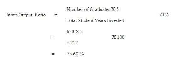
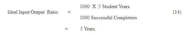
The above ratio indicates that the system is efficient to the extant of only 74 per cent and there is a scope of improvement and the wastage is of the tune of about 26 per cent. A ratio is said to be ideal, if it’s value is five in case of primary cycle. It may be recalled that we have started analysis with a hypothetical cohort of 1000 students which means the system should take at least five years to produce a primary graduate which otherwise gives an Input/Output ratio of 5. But in reality most of the systems have an Input/Output ratio well above the five. The Ideal Input/Output Ratio is defined as follows:
(ii) Input per Graduate
Now let us compute the actual Input/Output ratio which should be linked to number of student years invested and number of those who successfully complete an education cycle. One of the important indicators which reflect on wastage and efficiency of the education system is Input per Graduate, which means average number of years the system took to produce a graduate. Ideally a student should take five years to complete primary cycle and three years to middle cycle but the situation in reality is not so.
Box 5
Reconstructed Cohort Method : Flow of Students
Cohort 1990
| Grades | ||||||||||||||||||
| Year | I | II | III | IV | V | Input | ||||||||||||
| 83 | 83 | |||||||||||||||||
| 1990 | 1000 | 1000 | ||||||||||||||||
| 865 | ||||||||||||||||||
| 52 | ||||||||||||||||||
| 4 | 123 | 127 | ||||||||||||||||
| 1991 | 52 | 865 | 917 | |||||||||||||||
| 45 | 718 | |||||||||||||||||
| 3 | 24 | |||||||||||||||||
| 0 | 10 | 70 | 80 | |||||||||||||||
| 1992 | 3 | 69 | 718 | 790 | ||||||||||||||
| 3 | 57 | 625 | ||||||||||||||||
| 0 | 2 | 23 | ||||||||||||||||
| 0 | 1 | 7 | 42 | 50 | ||||||||||||||
| 1993 | 0 | 5 | 80 | 625 | 710 | |||||||||||||
| 0 | 4 | 70 | 557 | |||||||||||||||
| 0 | 3 | 26 | Output | |||||||||||||||
| 0 | 1 | 6 | 27 | 34 | ||||||||||||||
| 1994 | 0 | 7 | 96 | 557 | 660 | 506 | ||||||||||||
| 0 | 6 | 86 | ||||||||||||||||
| 0 | 4 | 24 | ||||||||||||||||
| 0 | 1 | 5 | 6 | |||||||||||||||
| 1995 | 0 | 10 | 110 | 120 | 100 | |||||||||||||
| 0 | 9 | |||||||||||||||||
| 0 | 5 | |||||||||||||||||
| 0 | 0 | 0 | ||||||||||||||||
| 1996 | 0 | 14 | 14 | 13 | ||||||||||||||
| 0 | ||||||||||||||||||
| 1 | ||||||||||||||||||
| 0 | 0 | |||||||||||||||||
| 1997 | 1 | 1 | 1 | |||||||||||||||
| Input | ||||||||||||||||||
| years | 1055 | 939 | 805 | 731 | 682 | 4212 | ||||||||||||
| Survival | ||||||||||||||||||
| by | 87 | 134 | 78 | 49 | 32 | |||||||||||||
| grades | 1000 | ——- | 913 | ——- | 779 | ——- | 701 | ——- | 652 | |||||||||
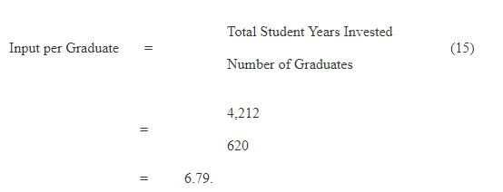
An Input/Output ratio of 6.79 indicates that the system is taking about 1.79 years more than the required five years which shows a wastage of about 26 per cent (1.79/6.79*100) which is similar to one presented above.
(iii) Wastage Ratio
Let us now compute one of the other important indicator of wastage, namely the Wastage Ratio. The ratio of actual Input/Output ratio to ideal Input/Output Ratio is termed as wastage ratio which always lies between 1 and ¥. In an ideal situation where the system has maximum efficiency, the ratio is one, otherwise more than one indicate extent of inefficiency and wastage. Thus, the ratio is computed as follows:
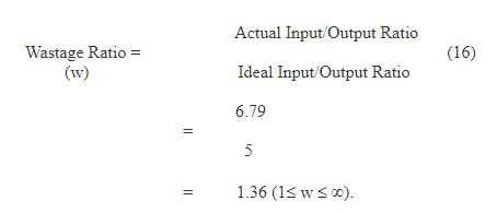
The wastage ratio computed above reveals that it is well above the ideal ratio i.e. one. The ratio also indicates that there is a scope of improvement in the system which can be handled efficiently, if complete information on wastage on account of drop‑outs and repeaters is available. Further, if the ratio is computed for different target groups would help us to identify where it is exorbitantly high and alarming. This can be checked through policy interventions and by improving efficiency.
(iv) Wastage on Account of Repeaters & Drop‑outs
In order to work out wastage on account of repeaters and drop‑outs, let us first analyse the evolution of cohort over a period of time. It is evident that of the total investment of 4,212 student years, graduates have consumed only 3,100 student years i.e. (620 x 5). Thus, the balance of 1,112 student years have gone waste which may be due to either repeaters or drop‑outs. Or in other words 1,112 more student years than required were used to produce 620 graduates. Let us first examine the break‑up of 620 graduates:
620 = 506 (5) + 100 (6) + 13 (7) + 1 (8)
The above equation reveals that of the total 620 graduates, only 506 students have taken exactly five years compared to 99 students who have taken six years, 13 students seven years and only 1 student has taken eight years. Thus, 100, 13 and 1 students have respectively taken 1, 2 and 3 years more than ideally required to become a primary graduate which is termed as wastage on part of repeaters. Thus,
100 x 1 + 13 x 2 + 1 x 3 = 129 students years were wasted. Similarly wastage on account of drop‑outs can also be worked‑out as follows:
83 x 1 + 127 x 2 + 80 x 3 + 50 x 4 + 34 x 5 + 6 x 6 + 0 x 7 + 0 x 8 = 983
Thus, the wastage on account of repeaters and drop‑outs comes out to be equal to total wastage i.e. 1,112 which can be used to compute percentage wastage on account of repeaters and drop‑outs as follows:
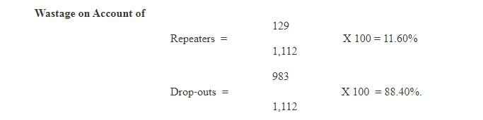
(v) Average Duration of Stay: Graduates, Drop‑out and Cohort
The next indicator of efficiency we present below is Average Duration of Stay in the system which can be computed separately for graduates, drop‑outs and also for entire cohort as a whole. The detailed computational procedure is presented below.
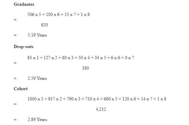
It may be noted that 620, 380 and 4,212 are number of graduates, drop‑outs and total student years invested during the entire evolution of hypothetical cohort of 1,000 students who entered into the system in the year 1990. The average stay in the system indicates that on an average a dropped‑out student stayed for at least 2.59 years which is slightly lower than the average stay for the entire cohort. Hence, drop‑outs have contributed a lot to wastage which is also evident from the percentage wastage on account of drop‑outs presented above.
(vi) Cohort Survival & Drop‑out Rates
The last indicator of efficiency based on hypothetical cohort method is cohort survival and drop‑out rates. The number of survivals and drop‑outs up to a particular grade can easily be obtained from the evolution of hypothetical cohort presented above in Box 5. The last two rows indicate that only 913 students remained in the system up to Grade II which is obtained by subtracting number of drop‑outs who left the system before reaching to Grade II from the initial 1,000 students in Grade I. Thus, giving cohort survival and drop‑out rate to be 8.70 per cent (87/1,000 X 100) and 91.30 per cent (913/1,000 X 100) respectively. Similarly, rates for the remaining grades can also be obtained. The cohort survival and drop‑out rates tell us in which grade is the drop‑out rate highest. The exercise can be repeated for different target groups. Once the grade and target group along with sub‑area which has lowest survival is identified, the next step is to initiate programmes, so that the survival rate is improved.
Some of the indicators of efficiency discussed above are computed at the all‑India level for three cohorts, namely 1985‑86, 1986‑87 and 1987‑88. The results are presented in Table 10. The perusal of results reveal that over a period of time, at primary level, the wastage ratio has declined from 1.45 in 1985‑86 to 1.44 in 1986‑87 which has further declined to 1.34 in 1987‑88. Similarly, a declining trend has been observed in number of years the system took to produce a primary graduate which is considered a healthy sign, however it is still on high side. The results further show that though the efficiency of the education system is improving but still around 34 per cent of the efforts are going waste which is also evident from the amount of wastage on account of repeaters and drop‑outs. Of the total wastage in 1987‑88, repeaters share was only 16.59 per cent compared to 83.41 per cent drop‑outs, relative figures for girls are 14.50 per cent and 85.50 per cent which show that girls tend to repeat less than their counterparts but preferred to drop‑out from the system which severely affect the efficiency of the education system. Unless this is checked, the efficiency of system at the primary level would continue be at low ebb. However, different studies suggest that this could not be possible by one single method or once for all action but it should involve the whole educational system. School community relationships, instructional material, curriculum, infrastructural facilities, quality of teaching and supervision are some of the areas where policy interventions may be required (NIEPA, 1992a).
Table 10
Efficiency of Education System: Primary Education
Selected Indicators: 1985‑86 to 1987‑88
| Cohort | Wastage | Input/ | Amount of Wastage | Average Duration of Study | |||
| Ratio | Graduate | on Account of | |||||
| (Years) | Repeaters | Drop-outs | Graduate | Drop‑outs | Cohort | ||
| Boys | |||||||
| 1985‑86 | 1.40 | 7.13 | 13.90 | 86.10 | 5.20 | 2.10 | 2.80 |
| 1986‑87 | 1.39 | 7.02 | 13.40 | 86.60 | 5.20 | 2.13 | 2.67 |
| 1987‑88 | 1.31 | 6.54 | 18.41 | 81.59 | 5.23 | 2.45 | 4.26 |
| Girls | |||||||
| 1985‑86 | 1.50 | 7.49 | 12.40 | 87.60 | 5.20 | 2.20 | 3.70 |
| 1986‑87 | 1.49 | 7.47 | 12.00 | 88.00 | 5.21 | 2.15 | 3.68 |
| 1987‑88 | 1.40 | 6.98 | 14.50 | 85.50 | 5.22 | 2.38 | 4.01 |
| Total | |||||||
| 1985‑86 | 1.45 | 7.25 | 13.40 | 86.60 | 5.20 | 2.20 | 3.70 |
| 1986‑87 | 1.44 | 7.20 | 12.80 | 87.20 | 5.20 | 2.14 | 3.67 |
| 1987‑88 | 1.34 | 6.71 | 16.59 | 83.41 | 5.22 | 2.42 | 4.16 |
Source: Mehta, Arun C. (1995a).
INDICATORS OF FACILITIES
Few indicators of quality of facilities and their utilisation is presented below. However, it may be noted that it is not an easy task to develop indicators of quality of facilities because of lack of precise definition of quality of education which is generally judged in terms of learners achievements (Kapoor, n.d.). The next important question one may ask is about factors which influence quality of education in general and learners achievement in particular. A large number of studies conducted in the recent past have identified a number of factors some of which can be grouped under the following two broad headings:
(a) School Buildings and Equipments Related Indicators; and
(b) Indicators Relating to Staffing Conditions.
(a) School Buildings and Equipments
As mentioned, the first stage of planning is diagnosis of the existing position which also includes school buildings and equipments which enables to answer a variety of questions. The first important objective of this exercise is to assess the availability of school buildings and also the quality of available buildings which plays an important role to identify priority areas, so that renovation and extension of buildings are taken up. The analysis of equipments will help to identify disadvantaged areas and will also help to assess true capacity of a school, so that schools which are underutilised or conversely overloaded can be identified (Kapoor, n.d.). Once the facilities are identified, the next important question is about their utilisation which should be compared in relation to national standards. So far as the utilisation of premises in a primary school is concerned, the simple indicators, such as, percentage of schools which work double shifts and rooms which are used double shifts be computed. In case of a middle and secondary school, Time Utilisation Rate may be computed which is presented in equation (17).
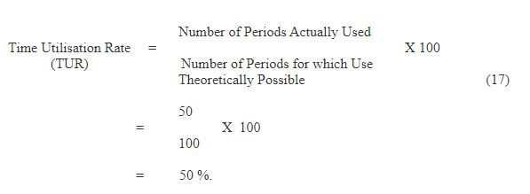
If Time Utilisation Rate for a particular school comes out to be 50 per cent which means that theoretically the school is in a position to allow 50 per cent additional enrollment even without improving the existing number of rooms. But, in practice this may or may not possible because of the contingencies of time‑table, the utilisation rate may not go beyond 90 per cent. One of the serious limitations of this indicator is that it fails to give any indication of how far room space is occupied (Kapoor, n.d.). For this purpose, Space Utilisation Rate (equation 18) may be used which relates average students who utilise room to its maximum capacity.
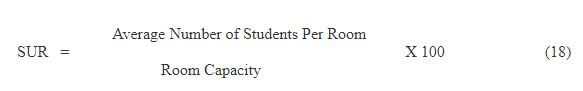
For example, ten rooms are built‑up in a school to accommodate about 1200 students but in reality the rooms on an average are occupied by only 600 students, which means SUR comes out to be only 50 per cent i.e.(600/1200* 100). The next important question which may crop‑up now is that for how much time the rooms are being utilised by these 50 per cent students for which Overall Utilisation Rate (equation 19) needs to be computed. Thus for the above data, the Overall Utilisation Rate comes out to be:
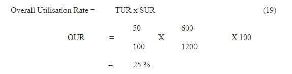
This rate should be used to asses utilisation of school premises which is based on both time and space utilisation, hence should be improved to the extent possible to decide adequacy of premises.
Needless to mention that the indicators presented above can be used only for micro level analysis.
(b) Equipments
The next set of indicators presented below relates to equipments and their utilisation. Generally, equipments cover furniture, teaching aids and educational supplies. Indicators of equipments of premises may be computed either school‑wise or classroom‑wise which depends upon the nature of a particular variable. Percentage of schools having electricity, drinking water and toilet facilities, playground and staff quarters are some of the basic indicators of facilities which can be computed for a block and district. But for facilities within schools, percentage of classrooms with pupils desk and teachers chair and table can be considered. So far as the teachers equipment is concerned, the same may be linked to scheme of Operation Blackboard in relation to timely supply of items, its adequacy and utilisation. Similarly, percentage of classrooms having blackboard may also be considered an indicator of teaching equipment, so as the percentage of teachers having maps, charts and globes. Percentage of children having textbooks, slates, exercise books and pencils are some of the indicators relating to pupil supplies. Similarly, percentage of children in a school receiving mid‑day meals, free textbooks and uniforms is an indicator of beneficiaries under a particular scheme.
(c) Staffing Conditions
Teacher plays an important role in functioning of school and imparting education. Therefore information on a number of variables, such as, qualifications, length of service, training, experience and subject needs to be collected. However, these factors themselves do not guarantee quality in a teacher, as it depends upon a number of other factors predominantly relating to working environment and type of school in which he/she works. Therefore, simple percentage distribution of teachers according to their education, sex and other variables mentioned above can be computed. The next area under which information needs to be collected is workload of teachers for which pupil‑teacher ratio and class‑size are calculated which can be used to know average audience. Class‑size is calculated by dividing total enrolment in a school to total number of classes in that school. But number of pupils being taught vary according to subject and teaching method and hence, class‑size may not always present true picture. Average Audience indicator is better indicator than the class‑size (Kapoor, n.d.) which consider average enrolment of the groups which is being taught by one teacher (equation 20). However, the indicator is recommended to compute at the institutional level only.
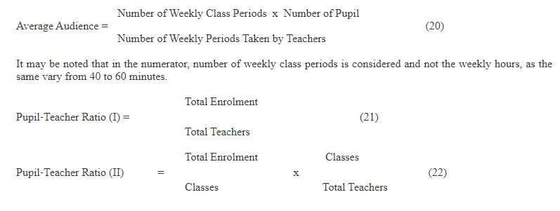
The other simple indicator of utilisation of teachers is Pupil‑Teacher Ratio (equation 21) which is simply a division of total enrolment to total teachers. In a more refined way, the ratio can also be computed by relating enrolment per class to classes per teacher. But in case of primary education, the teacher usually occupied with same class or classes, in that situation the indicator presented above in equation 22 will simply be the be Pupil‑Teacher Ratio (I). The detailed analysis of number of teachers in an institution according to subjects will reveal that the existing number of teachers is adequate or inadequate.
CONCLUSIONS
The indicators of educational development presented above are useful to undertake diagnosis of the existing situation. More specifically, the indicators of access, coverage, out‑of‑school children and drop‑out rate are used to identify educationally backward areas. However, one of the limitations of indicators based on the Reconstructed Cohort Method is that they do not take into account the quality of output that the system is producing. The method takes cognisance of only number of students who successfully complete an education cycle, which means learners attainment is totally ignored. The method also assumes that all the members of a cohort have identical facilities in schools, which may not always be true. Therefore, for comparing the efficiency of schools situated in the rural and urban areas and for the Government and Private schools, the method may not be appropriate to use. Government schools are practically open to all children irrespective of caste, creed, income and educational level of parents but the same is not true in case of the private schools. Admission test is one of the many considerations on the basis of which mostly children of the elite society used to get admission in the private schools. In contrast, only those children take admission in the Government schools whose parents do not have capacity to pay high tuition fee or alternatives to the Government schools are not available. Hence, an output of 700 out of 1000 input students may be considered efficient for a Government school but the same is not true for a school managed by the private organisation. Similarly, the socio‑economic background of students, if incorporated in the method would help to know whether the efficiency vary from one income group to another and educational level of parents. It may also be noted that the method takes into account only the number of drop‑outs and repeaters as possible causes of an inefficient system but ignores all other reasons which may pre‑dominantly relate to the delivery mechanism or the same may attribute to systems failure. May be, it is due to the medium of instructions which is not local or it is the teaching methods which are not effective or the infrastructure facilities are not adequate to retain children in the system. The method is also not suitable for the developed education systems, which have low drop‑out and repetition rate, and hence, it can be best applied to the systems, which have high incidence of drop‑out and repetition. Hence, the method needs further refinement.
REFERENCES
Johnstone, James N. (1981), Indicators of Educational Systems,
Kogan Page and UNESCO, London and Paris.
Kapoor, M.M. (n.d.), Indicators of Education, NIEPA New Delhi.
Kurrien, John (1983), Elementary Education in India, Myth, Reality and Alternative, Vikas Publishing House, New Delhi.
Mehta, Arun C. (1993a), `Education For All in India ‑ Myth and Reality’, Journal of Education and Social Change, Volume VI Number 3, December, pp 27‑68, Indian institute of Education, Pune.
Mehta, Arun C. (1993b), `A Survey of Estimates of Over‑age and Under‑age Children’, Journal of Education and Social Change, Number 2, Volume VII, July‑September, Pune.
Mehta, Arun C. (1994), `Efficiency and its Correlates : A Cross‑ State Analysis”, Journal of Perspectives in Education, Volume 10, Number 2, April, Baroda.
Mehta, Arun C. (1995a), Projections of Student Enrolment and Flow ‑ A Word Bank Sponsored Project, NIEPA, New Delhi, April.
Mehta, Arun C. (1995b), Education For All in India ‑Myth and Reality, Kanishka Publishers and Distributors, Delhi.
Mehta, Arun C. (1997a), `Enrolment and Teachers Projection Techniques, District Level Educational Planning, September, NIEPA, New Delhi.
Mehta, Arun C. (1997b), Data Requirements for Educational Planning: Limitations and Gaps in the Existing Information System, NIEPA, New Delhi.
Ministry of Human Resource Development (1986), National Policy on Education, Government of India, New Delhi.
Ministry of Human Resource Development (1987), The Scheme of Operation Blackboard, Government of India, New Delhi.
Ministry of Human Resource Development (1989), Report of the Working Group on Early Childhood Education and Elementary Education, New Delhi, Government of India.
Ministry of Human Resource Development (1992a), National Policy on Education : Programme of Action (Revised), Government of India, New Delhi.
Ministry of Human Resource Development (1992c), National Policy on Education, 1986 (Revised), Government of India, New Delhi.
Ministry of Human Resource Development (1992d), National Policy on Education : Programme of Action (Revised), New Delhi, Government of India.
Ministry of Human Resource Development (1993a), Education For All (The Indian Scene), Department of Education, Government of India, December, New Delhi.
Ministry of Human Resource Development (1993b), The District Primary Education Programme : Guidelines, Department of Education, Government of India, New Delhi.
Ministry of Human Resource Development (different years), Selected Educational Statistics, Department of Education, Government of India, New Delhi.
Ministry of Human Resource Development (different years), Education in India, Department of Education, Government of India, New Delhi
Ministry of Human Resource Development (different years), Annual Report, Government of India, New Delhi.
NCERT (1992), Fifth All India Educational Survey, Volume II, New Delhi.
NCERT (1995), Sixth All‑India Educational Survey: Provisional Statistics, November, New Delhi.
NIEPA, (1992), Report of Use of Sample Survey Techniques in Educational Statistics, Educational Planning Unit, New Delhi.
NIEPA (1993), National Sample Survey for Monitoring of UEE: 1990‑91, New Delhi.
NSSO (1991), Participation in Education, 42nd Round (July 1986‑ June 1987), Sarvekshana, Vol. XIV, No.3, Issue No.46, January‑March, Department of Statistics, Ministry of Planning, Government of India, New Delhi.
Planning Commission, (1992), Eighth Five Year Plan : 1992‑97 (Volume I & II), Objectives, Perspective, Macro‑Dimensions, Policy Framework and Resources, July, New Delhi, Government of India.
Prakash, Shri, Arun C. Mehta and SMIA Zaidi (1995), Indicators of Quality of Education: Conceptual and Methodological Thrusts, NIEPA, New Delhi.
Sapra, C.L. (1980), Demographic and Educational Statistics in India, Background Papers Presented at the Regional Training Seminar on Methods for Projecting School Enrolment in India, June 19 to July 12, 1978, NIEPA, New Delhi.
UNESCO (1982), Quantitative and Financial Aspects of Educational Planning (Book III), Basic Training Programme in Educational Planning and Management, UNESCO Regional Office for Education in Asia and the Pacific, Bangkok.
UNESCO, (1994), Use of Sample Survey Techniques in Educational Statistics, Current Survey and Research in Statistics, Paris.
Varghese, N.V. (1997), Modules on District Planning in Education, NIEPA, September, New Delhi.
Forty Years of Arun C Mehta at NIEPA: 1980 to 2019 (e-Book)
")
Times of India, New Delhi, 21st September 2021